CS 4495 / 6476 Project 2: Local Feature Matching
Interesting Points
Overview
The objective of this project is to find the matches between local features of two images. In general, the matching process can be divided into three steps: The first step is to find the corner points using a Harris corner detector, apply the threshold, and then pick the local maxima of each connected component. The second step is to calculate the SIFT descriptors for the interesting points. The final step is to calculate the feature differences and select point pairs according to the threshold ratio.
Find Interesting Points
To find the interesting points, we first need to preprocess the image pixels using Harris Detector. The method I used there is to filter the original image with the derivatives of small_Gaussian to get Ix and Iy. Then we need the larger_gaussian filter to calculate Ix2, Iy2 and Ixy.
% Step 0: Preparation: Set the variables and Gaussian filters

small_Gaussian = fspecial('gaussian', 3 .^ 2, 1);               	% small Gaussian
large_Gaussian = fspecial('gaussian', feature_width .^ 2, 2);   	% large Gaussian
[Guassian_dx, Guassian_dy] = gradient(small_Gaussian);          	% 1st derivitive of small_Gaussian
alpha = 0.04;                                                   	% alpha is between 0.04 and 0.06
img_size = size(image);                                         	% image size

% Step 1: Calculate the Ix, Iy, Ix2, Iy2, Ixy

Ix = imfilter(image, Guassian_dx);
Iy = imfilter(image, Guassian_dy);
Ix2 = imfilter(Ix .^ 2, large_Gaussian);
Iy2 = imfilter(Iy .^ 2, large_Gaussian);
Ixy = imfilter(Ix .* Iy, large_Gaussian);
The Harris's score of a point represents the distinction compared with its neighbors. Knowing Ix2, Iy2 and Ixy, I calculated Harris's score according to the following formula:
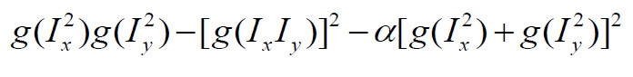
To get rid of the influence of the border points, I masked the harris matrix with the border matrix. Applied the threshold on the masked harris matrix. The threshold is adaptive according to the mean value of the masked harris matrix.
% Step 2: Calculate the harris value, apply the border and the thredshold
% on the result

harris = Ix2 .* Iy2 - Ixy .^ 2 - alpha .* (Ix2 + Iy2) .* (Ix2 + Iy2);
border = zeros(img_size);
border(feature_width + 1 : end - feature_width, feature_width + 1 : end - feature_width) = 1;
harris = harris .* border;
threshold = mean2(harris);
thresholded = harris > threshold;
Find the connected components and pick the local maxima of each component. The confidence is based on the harris score of each maxima.
% Step 3: Find the connected components, pick the local maximum and record
% the results to x, y and confidence.

cc = bwconncomp(thresholded);
num = cc.NumObjects;
x = zeros(num, 1);
y = zeros(num, 1);
confidence = zeros(num, 1);
img_size = size(image);
for idx = 1 : num
    pixels = cc.PixelIdxList{idx};
    component = harris(pixels);
    [maxNum, IDX] = max(component);
    [y(idx, 1), x(idx, 1)] = ind2sub(img_size, pixels(IDX));
    confidence(idx) = maxNum;
end
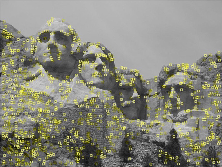
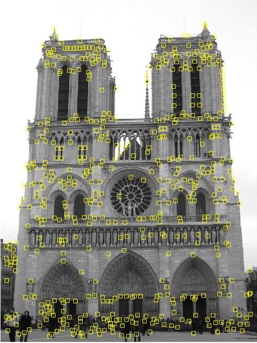
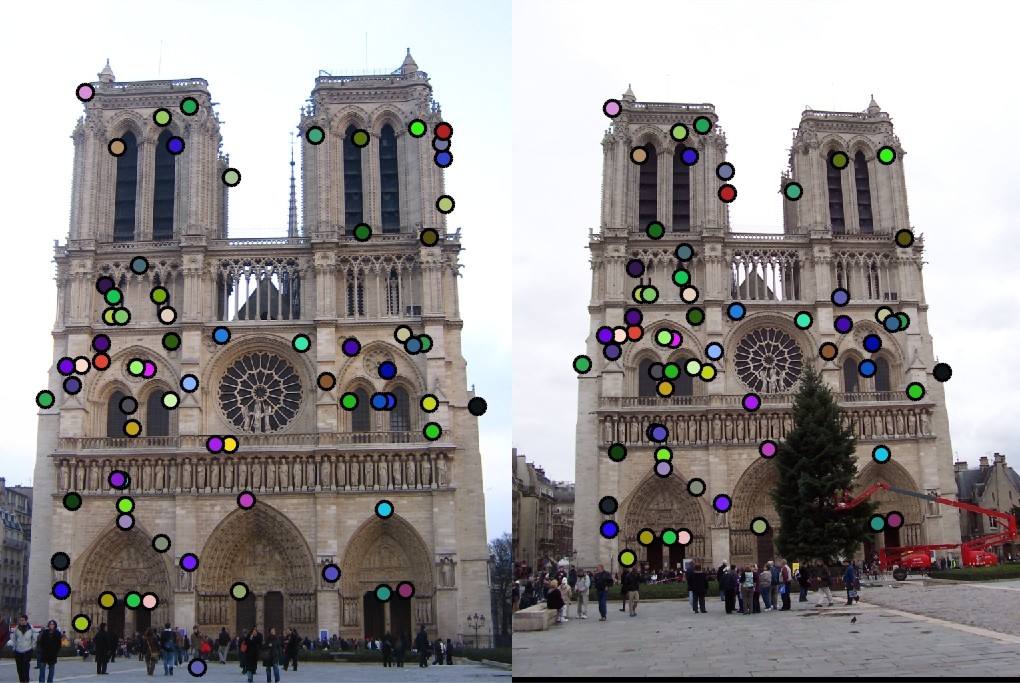
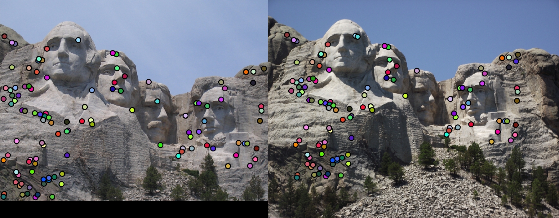
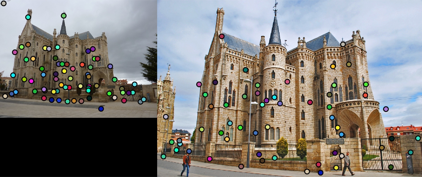
Figure 1: Interesting Points
Scaling(Extra):
As far as I am concerned, the scale is related to the average of the distances between intersting points. So I sum up the distances and then divide the square of the number of points by the sum to get the inverse of the scale. The scale will be used later on the feature_width during getting features.
% Step 4: Calculate the inverse of the scale
sum = 0;
for ii = 1: length(x)
    for jj = 2 : length(x)
        sum = sum + ((x(ii)-x(jj))^2 + (y(ii)-y(jj))^2)^(1/2);
    end
end
scale = (length(x) ^ 2) / sum;
Get Features according to Interesting Points
Apply the SIFT Algorithm to calculate the feature of each interseting point. The first step is to construct a 4 * 4 grid, of which each unit has 8 direction bins. Each bin is a magnitude representing the intensity of that direction. Thus for each interesting point, its feature is a 1 * 128 vector. To emphasize the importance of the close neighbors, I applied a gaussian filter with the same size of filter_width/2.
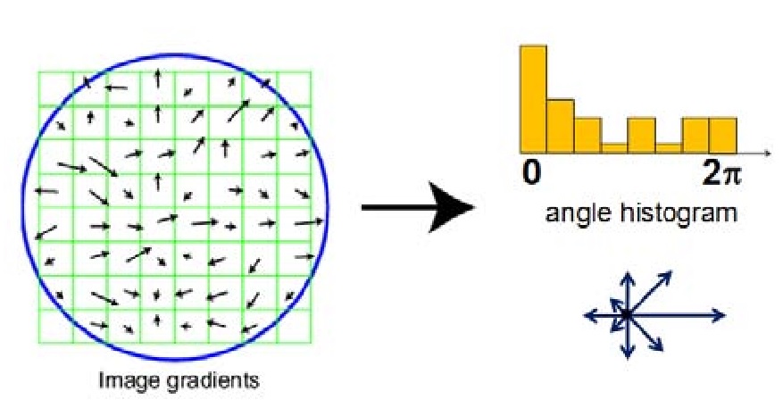
Figure 2: SIFT Process
Important Steps:
% Apply the scale
feature_width = round(feature_width  * scale / 4) * 4;

......

% Calculate the magnitude and direction of each pixel
magnitude = sqrt(Ix .^ 2 + Iy .^ 2);
direction = mod(round((atan2(Iy, Ix) + 2 * pi) / (pi / 4)), 8);

......

% Smooth the magitude matrix
large_mag_grid = magnitude(ys: ys + feature_width - 1, xs: xs + feature_width - 1);
large_dir_grid = direction(ys: ys + feature_width - 1, xs: xs + feature_width - 1);
large_mag_grid = imfilter(large_mag_grid, smooth_Gaussian);

......

% Normalize each feature
mag_sum = sum(features(point, :));
features(point, :) = features(point, :) / mag_sum;
Match the Features
The final step is to match the features. For each feature of image1, I calculated the distances between it and any feature form image2 and sort the result. The distance represents the similarity of the features and the radio of the smallest distance and the second small one represents the reliability. If the ratio is greater than a threshold, I picked the pair as a match.
Important Steps:
for i = 1 : size(features1, 1)
    distances = features2;
    for j = 1 : size(distances, 1)
        distances(j, :) = distances(j, :) - features1(i, :);
        distances(j, :) = distances(j, :) .^ 2;
    end
    [distList, index] = sort(sum(distances, 2));
    confidence = distList(2) / distList(1);
    if threshold > 1 / confidence
        matches(k, 1) = i;
        matches(k, 2) = index(1);
        confidences(k) = confidence;
        k = k + 1;
    end
end
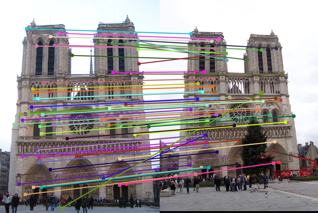
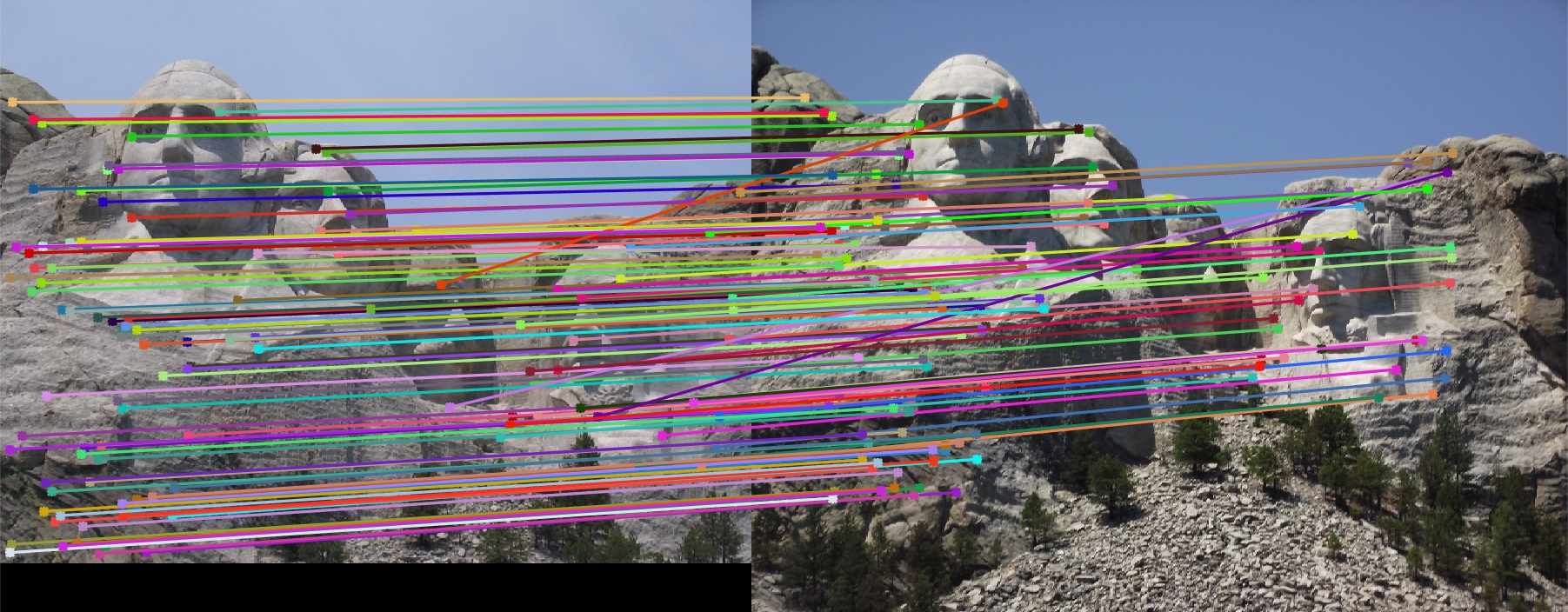
The matching results is acceptaable for Mount Rushmore and Notre Dame, while the accuracy is very low for Episcopal Gaudi before scaling. With the adaptive scaling, the accuracy is still around 30%. However, the scaling matching has more "close" pairs(not counted as correct match). This implies the performance is improved with scaling.
Table 1: Matching Results
 |
 |
| Notre Dame: Distance Ratio = 0.6 | 57 good matches; 14 bad matches; accuracy = 80% |
 |
 |
| Mount Rushmore: Distance Ratio = 0.6 | 110 good matches; 6 bad matches; accuracy = 95% |
 |
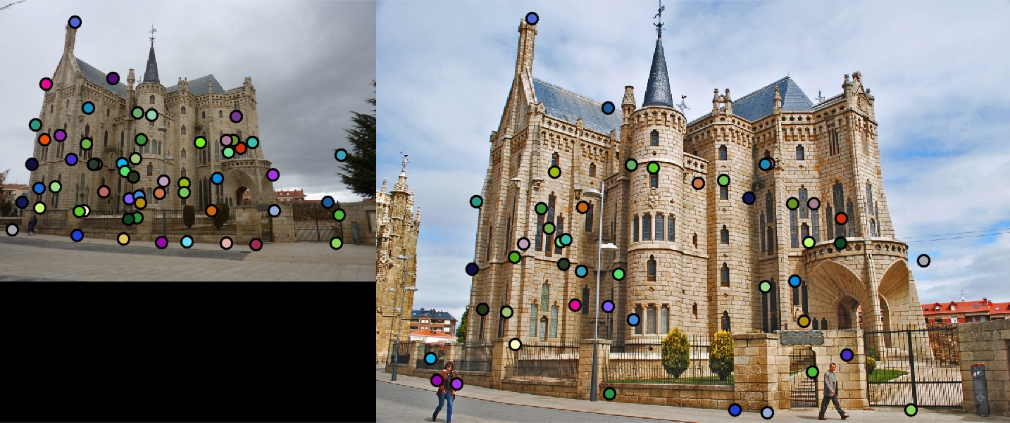 |
| Episcopal Gaudi (without scaling): Distance Ratio = 0.85; 3 good matches; 66 bad matches; accuracy = 4.3% | Episcopal Gaudi (with scaling): Distance Ratio = 0.85; 13 good matches; 44 bad matches; accuracy = 29.5% |
Conclusion
I am able to find the matches between images under some restriction. However, some pictures are not in the same scale, which leads to the low accuracy of the matchings. I implemented an easy way to find the scale of the image according to the average distance of the interesting points. This improved performance to some extent. On the other hand, the images may differ in the orientation. The orientation can be represented by the dominating edge direction, which can be calculated from the gradient. Rotate one of the image with the difference between dominating orientations should give a better performance.